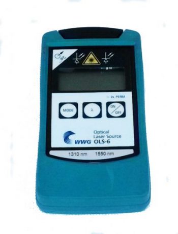
Calibration

Fiber optics

Our services

Fiber optical communications have transformed the telecommunication industry and have become the predominant choice for high-speed internet services and general data networking due to several advantages compared to communication over copper cables:

  • Fiber optic cables have much greater bandwidth than copper cables (i.e., higher Baud rate could be achieved, even more than 10-gigabit per strand).
  • Longer transmission distances are possible due to lower power loss (e.g., the longest recommended copper distance is 100 m while more than 10 GB/s could be achieved at over 40 km in length with optical fiber).
  • Fiber optic networks reduce the latency issues compared to cable Internet.
  • Optic cables are immune to electromagnetic interference therefore they are appropriate for electrically noisy environments and as such they can be used also for communication with the equipment in a shielded room where a strong electromagnetic field exist during EMC testing. Moreover, light signals from one fiber do not interfere with other fibers in the same fiber cable.
  • Optical fibers are smaller and lighter compared to copper wires (e.g., 30 times smaller cross-sectional area compared to copper wire), therefore more fibers can be bundled into a given-diameter cable.
  • Optical fibers usually have a longer life cycle for over 100 years.
  • Fiber optic cables are more secure since they do not radiate electromagnetic signals therefore the emissions cannot be intercepted while any attempts to penetrate the glass cable will cause “light leakage” which will cause noticeable degradation in communications which can be easily detected. Additionally, longer transmission distances allow hardware and electronics installation in one central location, unlike copper systems, where equipment needs to be installed within distribution locations.
  • Optical fibers are made of silica (i.e., SiO2) which is very abundant material therefore the optical fibers cost less than copper wires
  • Optical fiber has great tensile strength, they are flexible, bends easily and resists most corrosive elements.

Despite advantages over copper cable, the fiber optic cables also contain some drawbacks:

  • Optical fibers are more fragile and vulnerable to damage compared to copper wires. Fibers should not be twist or bend too tightly.
  • Optical fibers are difficult to splice.
  • Optical fibers are more expensive to install, as they must be installed by the specialists.
  • Fibers are less robust than copper wires.
  • Fiber optic cables are a small and compact thus they are highly susceptible to becoming cut or damaged during installation or construction activities.

Generally, three types of fiber optic cables exist:

  • Single mode optical fibers have a smaller core diameter of 9 μm and only allows a single wavelength of light to travel, which significantly decreases light reflections and lowers attenuation. These fibers are generally slightly more expansive than multimode fibers. They are often used in network connections over longer distances.
  • Multimode optical fibers have a larger core diameter than single mode cables, which allows multiple pathways and several wavelengths of light to be transmitted. Multimode optical fibers are available in 50 μm and 62.5 μm They are commonly used for shorter distances. According to the fiber refractive index distribution, multimode fiber can be divided into Step-Index Multimode Fiber and Graded-Index Multimode Fiber.
  • Plastic optical fibers are a large core step-index optical fibers with a typical 1 mm diameter. The larger diameter allows easier coupling of larger amount of light from sources and connectors that do not need to have high precision (lower cost, more durable, easier installation). Plastic optics is recommended for applications not requiring high bandwidth over great distances.

Wavelengths typically range from 800 nm to 1600 nm, but the most common wavelengths used in fiber optics are 850 nm, 1300 nm, and 1550 nm. Multimode fiber is designed to operate at 850 nm and 1300 nm, i.e., short wavelength, while single-mode fibers are optimized for 1550 nm and 1310 nm (less popular), i.e., long wavelength. Additionally, several different connectors exist. The most common are Bionic Connector (obsolete), Standard Connector SC, Ferrule Core Connector FC, ST Connector, SMA Connector, Lucent Connector LC, Plastic Fiber Optic Cable Connectors, Enterprise Systems Connection Connector ESCON, Fiber Distributed Data Interface Connector FDDI, Opti-Jack Connector, LX-5 Connector, Volition Connector, MT-RJ Connector, MU Connector, MT Connector, and E2000 Connector. Connectors are also available with differently polished end faces, which impact the connector’s level of return loss, i.e., the back reflection. The connectors are available either as a UPC (Ultra Physical Contact, connectors are colored blue) or an APC (Angled Physical Contact/Angled Polish Connector, i.e., 8° angle at the end face decreases the return loss, connectors are colored green). These connector types are not interchangeable due to the angle of an APC connector, so it is very important to verify the required connectors.

Fiber optics related metrology is quite like RF&MW metrology. The light is generated by optical laser source where the wavelength and optical power and linearity are parameters of importance. This is very similar to function generators and signal generators in RF&MW metrology where the frequency and generated power (voltage) are the main parameters of interest. The light is transited through optical fibers, optical splitters, and optical attenuators which acts like electrical cables, splitters and attenuators used in RF&MW metrology; in both cases the attenuation is the most important parameter of interest. The power is measured by optical power meter like power sensors in RF&MW metrology. The optical network could be diagnosed by optical time domain reflectometer OTDR which have similar function as vector network analyzer (VNA). Finally, a special attention on should be paid to different connector types (especially for UPC and APC connectors) and cleanness of the contacts. On contrary, a special attention should be taken on connector pin depth when dealing with different RF&MW connectors as well as different types of connectors (e.g., N-type connector for 50 Ω and 75 Ω looks very similar but the pins have different dimensions).

At SIQ we calibrate optical laser sources, optical power level meters, optical fibers, optical attenuators, and optical time domain reflectometers OTDRs. The calibration could be performed only on equipment that is based on 1310 nm and 1550 ns single mode 9 μm optical fibers equipped with FC/PC or SC/PC connectors.

Calibration of test equipment at SIQ

Laser power source

The calibrated parameter is absolute optical power level of laser power source which can be measured at different output levels (linearity) using reference laser power meter. The power can be measured in a 0 dBm to –90 dBm power range.

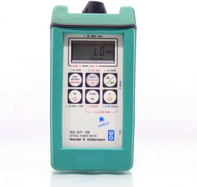
Optical power meters

We calibrate the absolute accuracy of optical power metes by comparison method using the reference optical power meter. Another parameter of importance is optical power level linearity which is calibrated using a reference optical attenuator. The power can be measured in 0 dBm to –90 dBm power range.

Optical attenuators and optical fibers

The main parameter of interest in both cases is optical insertion loss and (incremental and/or stepped) attenuation of optical step attenuators. The attenuation can be measured in 0 dB to 90 dB range by comparison method (uncertainties from 0.15 dB to 0.17 dB) or by method using variable optical attenuator in –1.4 dB to –60 dB range (uncertainties 0.06 dB). We can also calibrate optical length of optical fiber at known group refractive index (distances from 0.1 km to 100 km).

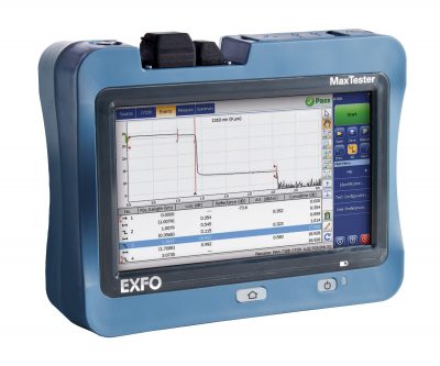
Optical time domain reflectometers (OTDRs)

OTDR is an instrument that can measure distance to certain events (connectors, splices, or faults) and attenuation in optical fiber. This is done by sending a laser light pulse into the optical fiber and then measuring the backscattered signal from the fiber in given time intervals. The scattering is either Rayleigh scattering on the micro particles in the optical fiber glass or Fresnel refraction which takes place at boundaries between different materials in the path of the light pulse (connectors, splices, etc.). If group refractive index of the fiber is known, then the distance to given event can be calculated using the time when this signal was received. The level of the received signal is a measure of fiber attenuation, thus the OTDR can also measure the loss of optical power in the fiber. Typical parameters that we calibrate are:

  • loss scale in region A, ΔSA (typical fiber trace ± 3 dB per km distance, 0 km to 35 km)
  • distance offset error, ΔL0, is the displayed location of the OTDR’s front panel connector (ideally, the displayed location should be zero)
  • distance scale error, ΔSL, is the error of the distance slope (it can be measured from 5 km to 35 km)
  • loss scale calibration (loss scale calibration is used to determine the accuracy of the loss measurement ΔSA of an OTDR, for power levels F within the OTDR’s backscatter regime)
  • event deadzone (the event deadzone is usually specified for a pulse width of 1 μs and a reflectance of –35 dB unless otherwise stated in the specifications)
  • attenuation deadzone (the attenuation deadzone is defined as the displayed difference between the beginning of a reflection to the point where the signal returns to the backscatter trace within a given error band, at a given reflectance)
  • dynamic range (The dynamic range characterizes the OTDR’s ability to measure long fibers and, accordingly, small backscatter signals. It is defined as the difference between the extrapolated start of the backscatter trace and the noise level, expressed in dB of one-way fiber loss.)

Contact us

Interested more? Contact our team of experts.

Write to us

  • SIQ Ljubljana